Hedonic Home Price Prediction in Boston, MA
Guy Duer
January 4, 2018
Introduction
(This fictional report was prepared as a class assignment for MUSA507 at the University of Pennsylvania)
My client, Zillow, has realized that the predictions of home prices in the Boston area which are currently on the site are not sufficiently accurate. This lack of accuracy is putting the site’s credibility in question and hurting its ability to attract and retain customers in the region.
Accurately predicting home prices is difficult. Home prices are a function of many complex considerations including the physical characteristics, location, and other factors including seasonal variations and the personal preferences of buyers and sellers.
To achieve better prediction accuracy, I have collected data to capture as many of the factors listed above as possible. More specifically, I worked to capture the variation in prices due to both physical characteristics of homes, and the underlying spatial patterns of prices in the region.
The resulting model was able to improve predictions considerably, with a new error margin of only about 11%-12%.
The map below shows the observation points in the data set.
library(dplyr)

options(scipen=999)

df <- read.csv("WrangledData.csv")
df2 <- select(df, -Parcel_No, -Latitude_1, -Longitud_1)
df$SalePrice <- sapply(df$SalePrice, as.numeric)

df_Train <- df2[df2$SalePrice > 0,]

df_Test <- df2[df2$SalePrice == 0,]
library(leaflet)
leaflet(data = df) %>% setView(lng = -71.08, lat = 42.33, zoom = 12) %>% addProviderTiles(providers$CartoDB.Positron) %>%
addProviderTiles(providers$Stamen.TonerLines, options = providerTileOptions(opacity = 0.35)) %>%
addProviderTiles( providers$Stamen.TonerLabels) %>%
addCircleMarkers(lng = df$Longitud_1, lat = df$Latitude_1, radius = 3, color = ifelse(df$SalePrice > 0, "blue", "red"), stroke = FALSE, fillOpacity = 0.5, clusterOptions = markerClusterOptions(disableClusteringAtZoom = 13), label = ~as.character(paste("Sale Number: ", UniqueSale, ", " ,"Sale Price: $", SalePrice))) %>%
addLegend("topright", colors = c("red", "blue"), labels = c("Test-Set", "Training-Set"),
title = "Training/Testing Set",
opacity = 1
)Data
Data variables came from various sources. Physical housing characteristics, and the sales date were provided in the original Zillow data set. Some variables from the original data set with many categorical values or uneven distribution of values (e.g. sale date, year remodeled) were modified in order to increase predictive capacity.
New variables which model spatial considerations were added to the data set. These variables were created through spatial analyses of the original data set, as well as through the incorporation of data gathered from open data sources on the web.
Summary Statistics
Description of the variables is available in the Appendix.
library(stargazer)
stargazer(df_Train, type="text", title = "Variable Summary Statistics")
##
## Variable Summary Statistics
## ===================================================================
## Statistic N Mean St. Dev. Min Max
## -------------------------------------------------------------------
## UniqueSale 1,323 739.166 428.927 1 1,485
## SalePrice 1,323 642,335.000 565,859.000 200,000 11,600,000
## LivingArea 1,323 2,310.966 993.217 573 9,908
## LAND_SF 1,323 4,562.249 3,382.821 498 63,941
## YR_BUILT 1,323 1,916.409 30.242 1,802 2,013
## YR_REMOD 1,323 749.477 968.163 0 2,013
## Last_Work 1,323 1,951.161 45.022 1,830 2,013
## NewlyRemodeled 1,323 0.138 0.345 0 1
## GROSS_AREA 1,323 3,622.726 1,422.172 826 11,919
## LIVING_ARE 1,323 2,280.961 994.508 573 9,908
## NUM_FLOORS 1,323 2.187 0.646 1.000 4.000
## R_TOTAL_RM 1,323 9.760 3.766 3 21
## R_BDRMS 1,323 4.494 2.008 1 14
## R_FULL_BTH 1,323 1.995 0.894 1 8
## R_HALF_BTH 1,323 0.363 0.547 0 3
## R_KITCH 1,323 1.697 0.822 1 4
## R_FPLACE 1,323 0.407 0.758 0 5
## ZIPCODE 1,323 2,128.682 16.894 2,108 2,467
## PTYPE 1,323 103.912 34.071 101 985
## OWN_OCC 1,323 0.559 0.497 0 1
## HEAT_SYS 1,323 0.986 0.116 0 1
## C_AC 1,323 0.145 0.352 0 1
## FeetToParks 1,323 492.798 353.428 3 1,964
## WalkScore 1,323 85.565 5.534 70 98
## TransitSco 1,323 68.864 14.870 44 100
## BikeScore 1,323 65.729 12.547 53 95
## FeetToMetro 1,323 5,674.466 4,965.023 187 19,768
## MEDHHINC 1,323 73,351.130 30,775.610 9,756 166,375
## PCTBACHMOR 1,323 39.403 22.517 0 97
## PCTOWNEROC 1,323 44.602 22.840 0 96
## PCTVACANT 1,323 4.594 3.061 0 28
## PCTWHITE 1,323 59.865 31.201 2 100
## CrimeIndex 1,323 3.964 1.931 1.000 9.610
## NearUni 1,323 0.168 0.374 0 1
## SchoolGrade 1,323 3.125 1.711 1 9
## DistToCBD 1,323 25,517.900 12,816.110 2,231 52,892
## NearImpBldg 1,323 0.011 0.106 0 1
## NearCommonwealth 1,323 0.003 0.055 0 1
## DistToPoor 1,323 3,610.567 3,149.793 0 15,573
## NearAP 1,323 0.021 0.144 0 1
## Ave_SalePr 1,323 638,684.900 447,084.200 283,541 4,470,000
## Dist_AP 1,323 31,408.400 14,682.450 2,894.213 57,307.500
## Dist_SC 1,323 2,164.640 942.232 420.376 4,909.092
## Dist_Major_Road 1,323 2,720.628 2,543.041 3.011 15,749.200
## -------------------------------------------------------------------Correlation Matrix
Avoiding multi-collinearity (high level of correlation between predictors) can help improve the accuracy of the model. To examine this, The correlation matrix of the numeric variables in the model is shown below. Variables with correlation greater than 0.8 will be removed from the model.
dfNum <- select(df_Train, -UniqueSale, -SaleSeason, -STRUCTURE_, -R_BLDG_STY, -SaleMonth, -Style , -LU, -R_ROOF_TYP, -HEAT_SYS, -R_EXT_FIN, -Neighborhood)

#Correlation Matrix
CorMatrix <- cor(dfNum)

library(corrplot)
corrplot(CorMatrix, method = "color", order = "AOE", addCoef.col="grey", type = "upper", addCoefasPercent = FALSE, number.cex = .7)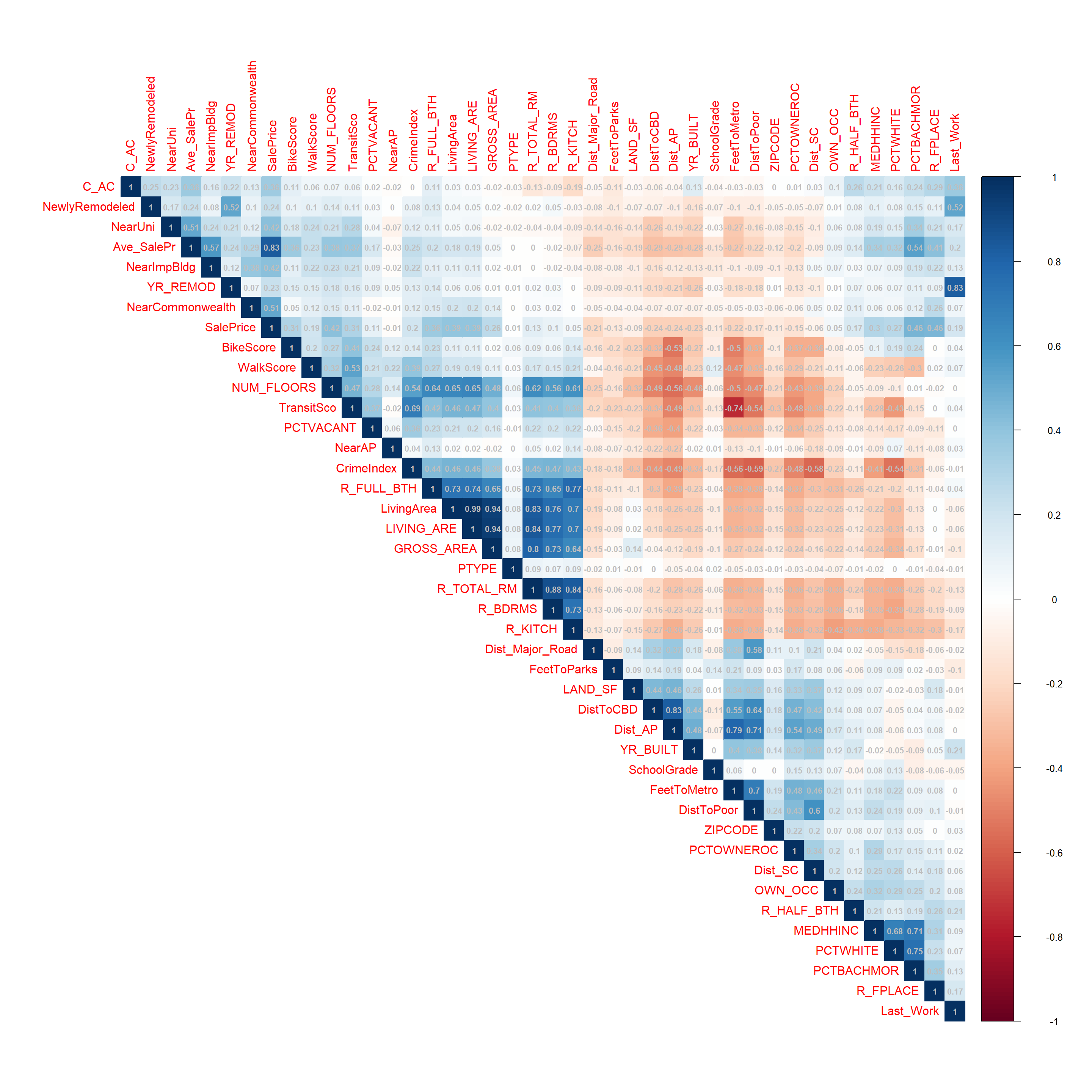
#Removing multi-colinear variables (>.80)
df2 <- select(df2, -GROSS_AREA, -LivingArea, -YR_REMOD, -R_BDRMS, -R_KITCH, -Dist_AP)
df_Train <- df2[df2$SalePrice > 0,]
df_Test <- df2[df2$SalePrice == 0,]
Analyzing Predictor Distributions
The OLS model works best when the predictors and dependent variable are normally distributed. The distribution of some predictors may be brought closer to a normal distribution by log-transforming them. The plots below show the current distributions of the continuous predictors.
#Analysis of continuous predictors
dfCont <- select(dfNum, -GROSS_AREA, -LivingArea, -YR_REMOD, -NewlyRemodeled, -R_BDRMS, -R_KITCH, -Dist_AP, -NearCommonwealth, -NearImpBldg, -NearUni, -C_AC, -OWN_OCC, -PTYPE, -ZIPCODE,
                 -R_FPLACE, -R_HALF_BTH, -R_FULL_BTH, -NearAP)

#Distribution analysis
library(reshape2)
dfContMelted <- melt(dfCont)

library(ggplot2)
ggplot(data = dfContMelted, mapping = aes(x = value)) +
  geom_histogram(bins = 30) + facet_wrap(~variable, scales = 'free_x') + theme(axis.text.x = element_blank())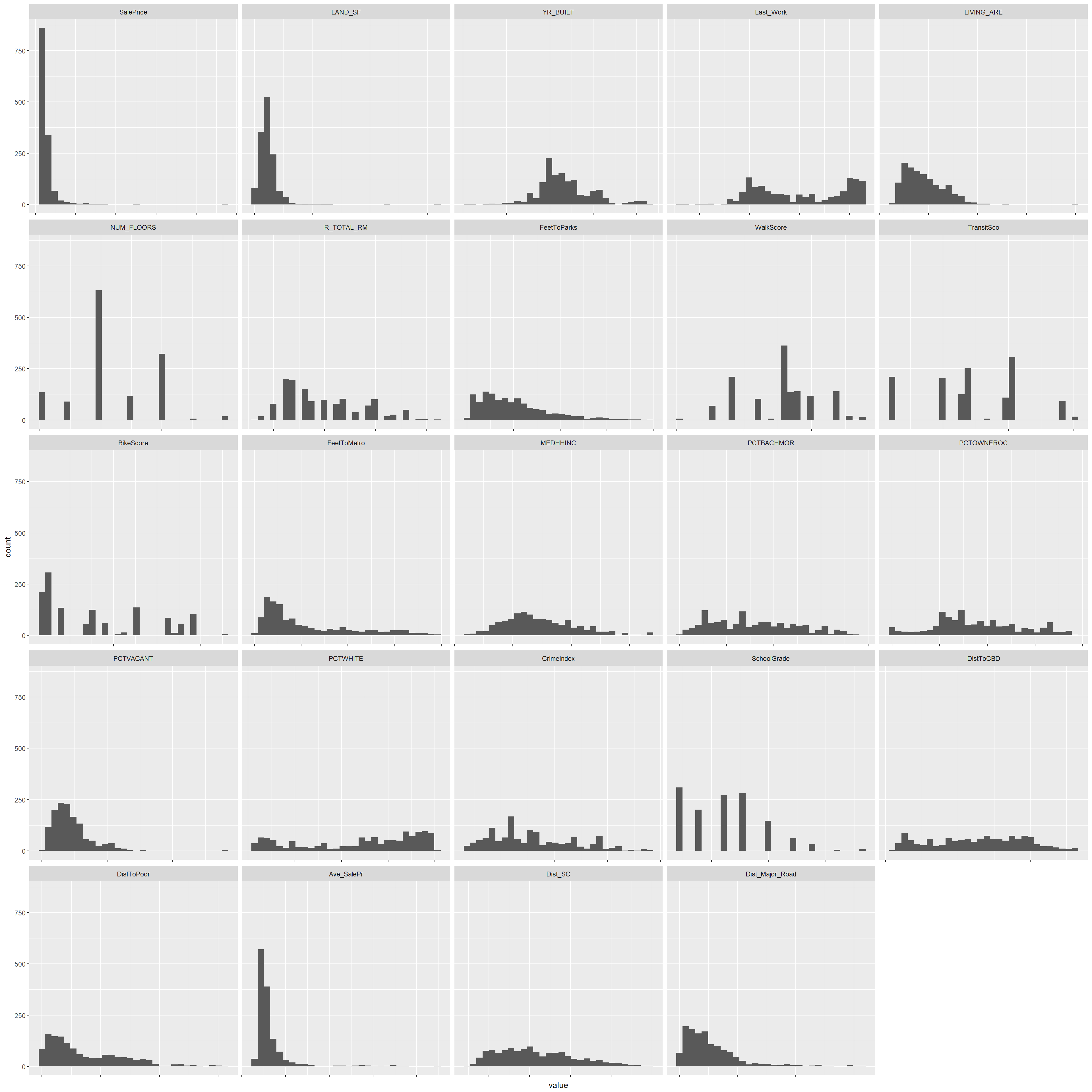
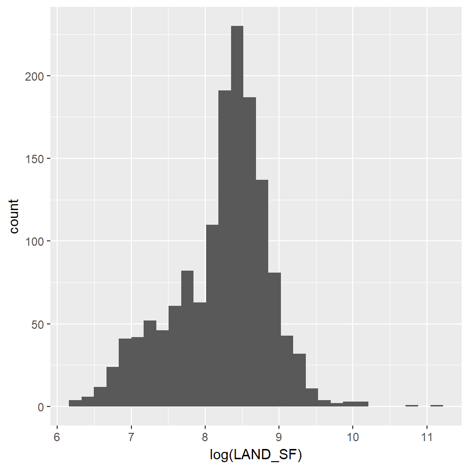
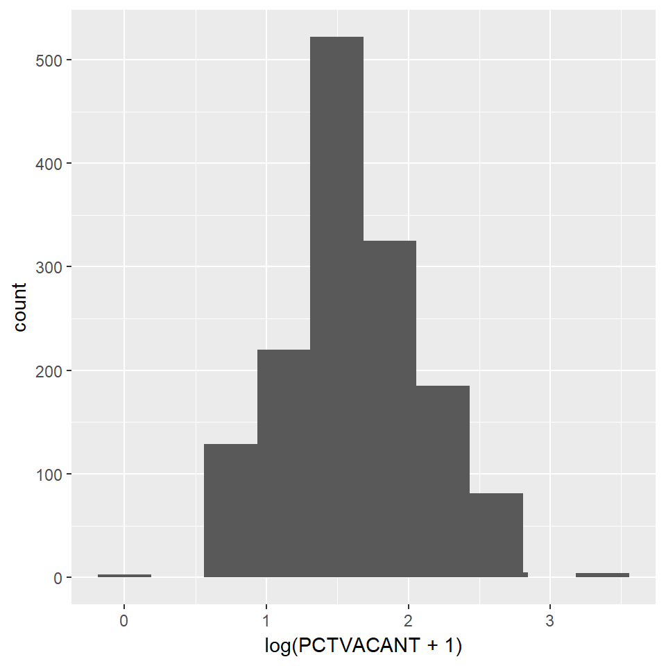
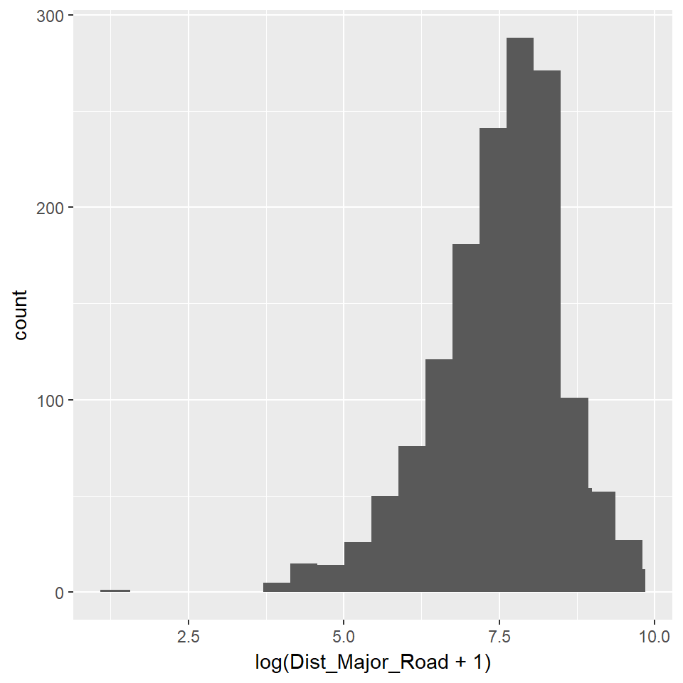
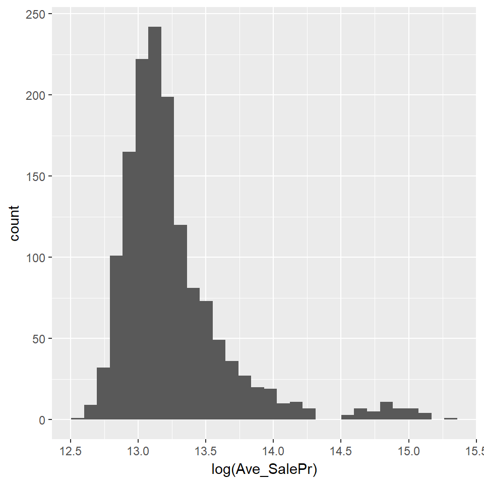
Predictors which are negatively skewed are the best candidates for normalizing by using log-transformation. The new distributions of the transformed predictors are shown below.
#Log-Transforming to normalize selected predictors
ggplot(df2, aes(x=LAND_SF)) + geom_histogram()
ggplot(df2, aes(x=log(LAND_SF))) + geom_histogram()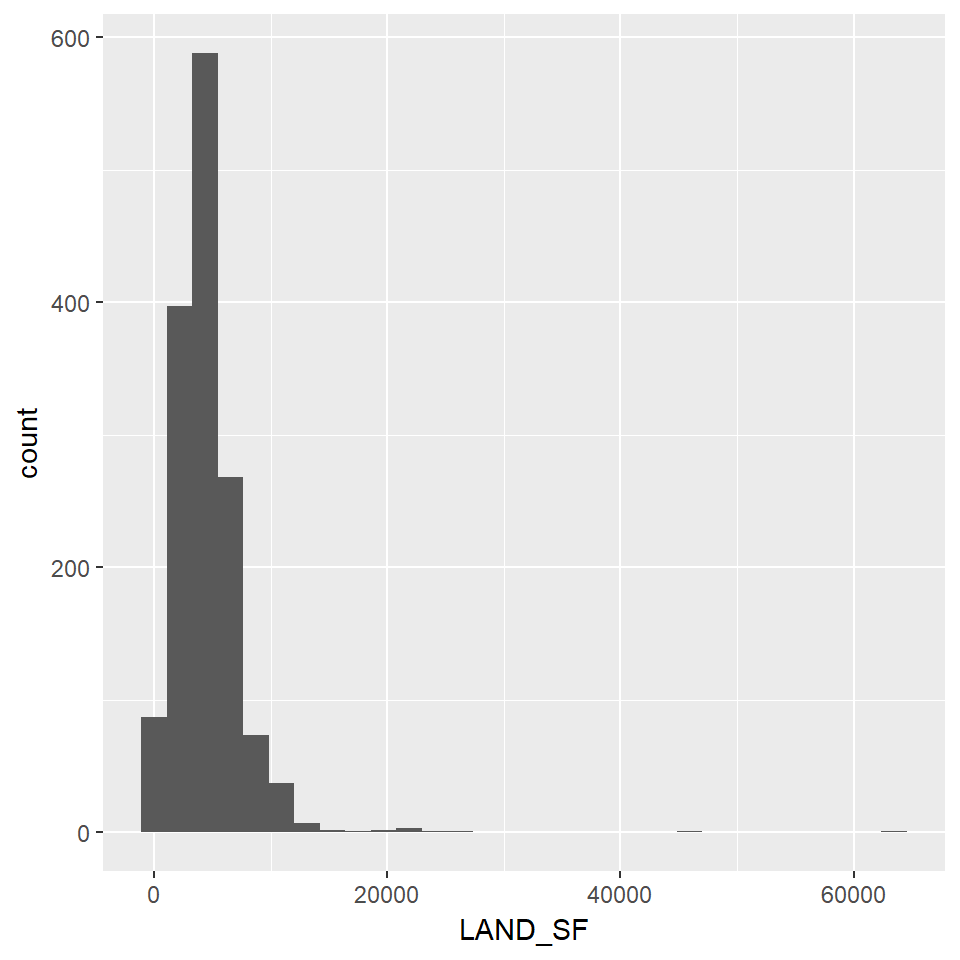
#Log-Transforming to normalize selected predictors
ggplot(df2, aes(x=LIVING_ARE)) + geom_histogram()
ggplot(df2, aes(x=log(LIVING_ARE))) + geom_histogram()

#Log-Transforming to normalize selected predictors
ggplot(df2, aes(x=PCTVACANT)) + geom_histogram() + stat_bin(bins = 10)
ggplot(df2, aes(x=log(PCTVACANT + 1))) + geom_histogram() + stat_bin(bins = 10)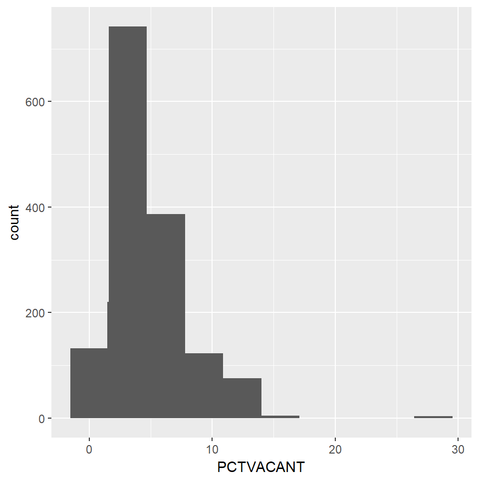
#Log-Transforming to normalize selected predictors
ggplot(df2, aes(x=Dist_Major_Road)) + geom_histogram() + stat_bin(bins = 20)
ggplot(df2, aes(x=log(Dist_Major_Road + 1))) + geom_histogram() + stat_bin(bins = 20)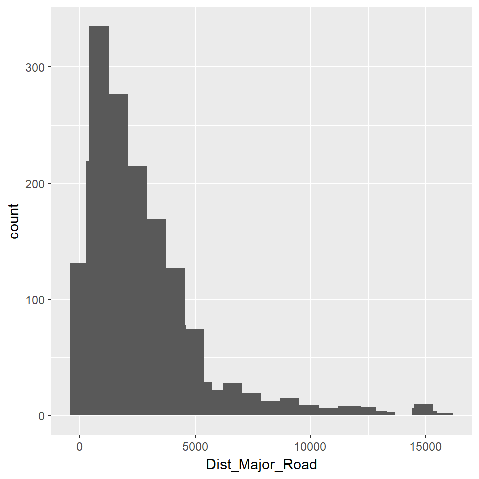
#Log-Transforming to normalize selected predictors
ggplot(df2, aes(x=Ave_SalePr)) + geom_histogram() + stat_bin(bins = 30)
ggplot(df2, aes(x=log(Ave_SalePr))) + geom_histogram() + stat_bin(bins = 30)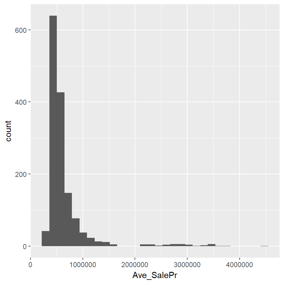
Methods
To generate the price predictions, I will use a Hedonic OLS Regression model. This method evaluates the direction and strength of the relationship between the dependent variable in question (home prices) and the many factors (predictors) which may affect it. The model can estimate the effect of each of our predictors on sale prices while holding all other predictors constant, thereby allowing us to consider the effect of different variables concurrently.
To train the model, I created a training data set (data set with known sale prices) which included 1323 observations to “train” the regression model to predict the home sales price in the test data set (the data set of homes with unknown, or 0, prices). Using this training data, it is possible to calibrate the regression coefficients to model home prices based on the data. Lastly, I used this “trained” model to predict the sale prices in the test set.
In evaluating the predictive ability of our model, I took two separate approaches. The first approach was “In-sample training”, in which I divided the training data-set into two groups, and used one of the groups to predict the prices in the other. The second approach was a 10-fold cross-validation algorithm, which randomly divids the training set into ten equal “folds”, and one by one predicts prices for each of the folds using the remaining nine folds.
To examine whether the model was sufficiently capturing spatial structure of prices, I used the Moran’s I method. This method evaluates whether the model’s errors are clustered in space to a statistically-significant degree (which would indicate some spatial dynamic that was not accounted for in the model).
Model Building
The model-building process is shown below.
Linear Regression model 1: All predictors
reg1 <- lm(log(SalePrice) ~ ., data =  df_Train %>%
             as.data.frame %>% dplyr::select(-UniqueSale))
Stepwise Variable Analysis:
step$anova## Stepwise Model Path
## Analysis of Deviance Table
##
## Initial Model:
## log(SalePrice) ~ YR_BUILT + Last_Work + NewlyRemodeled + NUM_FLOORS +
## R_TOTAL_RM + R_FULL_BTH + R_HALF_BTH + R_FPLACE + SaleSeason +
## SaleMonth + Style + ZIPCODE + PTYPE + OWN_OCC + LU + STRUCTURE_ +
## R_BLDG_STY + R_ROOF_TYP + R_EXT_FIN + HEAT_SYS + C_AC + FeetToParks +
## Neighborhood + WalkScore + TransitSco + BikeScore + FeetToMetro +
## MEDHHINC + PCTBACHMOR + PCTOWNEROC + PCTWHITE + CrimeIndex +
## NearUni + SchoolGrade + DistToCBD + NearImpBldg + NearCommonwealth +
## DistToPoor + NearAP + Dist_SC + LogLAND_SF + LogLIVING_ARE +
## LogPCTVACANT + LogDist_Major_Road + LogAve_SalePr
##
## Final Model:
## log(SalePrice) ~ Last_Work + NewlyRemodeled + NUM_FLOORS + R_FULL_BTH +
## R_HALF_BTH + R_FPLACE + SaleMonth + Style + PTYPE + LU +
## R_BLDG_STY + R_EXT_FIN + C_AC + Neighborhood + FeetToMetro +
## PCTBACHMOR + PCTWHITE + CrimeIndex + NearUni + NearImpBldg +
## NearAP + Dist_SC + LogLAND_SF + LogLIVING_ARE + LogAve_SalePr
##
##
## Step Df Deviance Resid. Df Resid. Dev
## 1 1216 28.71204
## 2 - BikeScore 0 0.0000000000000000000 1216 28.71204
## 3 - TransitSco 0 0.0000000000000000000 1216 28.71204
## 4 - WalkScore 0 0.0000000000000000000 1216 28.71204
## 5 - SaleSeason 0 0.0000000000003552714 1216 28.71204
## 6 - R_ROOF_TYP 5 0.0946874920781439755 1221 28.80673
## 7 - STRUCTURE_ 2 0.0358108356566724240 1223 28.84254
## 8 - FeetToParks 1 0.0000047751824361342 1224 28.84254
## 9 - R_TOTAL_RM 1 0.0000139125347544677 1225 28.84256
## 10 - LogDist_Major_Road 1 0.0001061660543335563 1226 28.84266
## 11 - PCTOWNEROC 1 0.0002904673328529839 1227 28.84296
## 12 - MEDHHINC 1 0.0008064345835343545 1228 28.84376
## 13 - OWN_OCC 1 0.0030725642581721502 1229 28.84683
## 14 - HEAT_SYS 1 0.0059915654671662821 1230 28.85283
## 15 - DistToCBD 1 0.0138947193882579256 1231 28.86672
## 16 - YR_BUILT 1 0.0138758735296633517 1232 28.88060
## 17 - LogPCTVACANT 1 0.0151253646420634880 1233 28.89572
## 18 - SchoolGrade 1 0.0202790166078798961 1234 28.91600
## 19 - DistToPoor 1 0.0214955404639987080 1235 28.93750
## 20 - ZIPCODE 1 0.0265304549993281569 1236 28.96403
## 21 - NearCommonwealth 1 0.0328592482080054538 1237 28.99689
## AIC
## 1 -4853.541
## 2 -4853.541
## 3 -4853.541
## 4 -4853.541
## 5 -4853.541
## 6 -4859.185
## 7 -4861.541
## 8 -4863.541
## 9 -4865.540
## 10 -4867.535
## 11 -4869.522
## 12 -4871.485
## 13 -4873.344
## 14 -4875.069
## 15 -4876.432
## 16 -4877.797
## 17 -4879.104
## 18 -4880.176
## 19 -4881.193
## 20 -4881.980
## 21 -4882.480linear regression model 2- Removing highly insignificant predictors:
reg2 <- lm(log(SalePrice) ~ ., data =  df_Train %>%
             as.data.frame %>% dplyr::select(-UniqueSale, -PCTOWNEROC, -DistToPoor,
                                             -DistToCBD, -SchoolGrade, -MEDHHINC, -WalkScore, -TransitSco,
                                             -BikeScore, -FeetToParks, -HEAT_SYS, -R_EXT_FIN, -R_BLDG_STY, -R_ROOF_TYP, -STRUCTURE_,
                                             -OWN_OCC, -ZIPCODE, -Style, -SaleMonth))
linear regression model 3- Removing more insignificant predictors:
library(stargazer)
reg3 <- lm(log(SalePrice) ~ ., data =  df_Train %>%
             as.data.frame %>% dplyr::select(-UniqueSale, -LogDist_Major_Road, -PCTOWNEROC, -DistToPoor,
                                             -DistToCBD, -SchoolGrade, -MEDHHINC, -WalkScore, -TransitSco,
                                             -BikeScore, -FeetToParks, -HEAT_SYS, -R_EXT_FIN, -R_BLDG_STY, -R_ROOF_TYP, -STRUCTURE_,
                                             -OWN_OCC, -ZIPCODE, -Style, -SaleMonth, -YR_BUILT, -R_TOTAL_RM, -NearImpBldg, -NearCommonwealth,
                                             -NearCommonwealth, -LogPCTVACANT))


stargazer(reg1, reg2, reg3, type="text", title = "Model Outputs", align=TRUE, no.space=TRUE, single.row=TRUE, ci=FALSE, column.labels=c("Model 1","Model 2", "Model 3"))
##
## Model Outputs
## ==========================================================================================================
## Dependent variable:
## --------------------------------------------------------------------------------
## log(SalePrice)
## Model 1 Model 2 Model 3
## (1) (2) (3)
## ----------------------------------------------------------------------------------------------------------
## YR_BUILT 0.0001 (0.0002) 0.00003 (0.0002)
## Last_Work 0.0003** (0.0001) 0.0004*** (0.0001) 0.0003*** (0.0001)
## NewlyRemodeled 0.045*** (0.016) 0.038** (0.016) 0.040*** (0.016)
## NUM_FLOORS 0.036* (0.019) 0.064*** (0.014) 0.064*** (0.014)
## R_TOTAL_RM -0.0004 (0.003) -0.001 (0.003)
## R_FULL_BTH 0.044*** (0.010) 0.046*** (0.010) 0.047*** (0.010)
## R_HALF_BTH 0.024** (0.010) 0.018* (0.010) 0.020** (0.010)
## R_FPLACE 0.038*** (0.008) 0.044*** (0.008) 0.045*** (0.007)
## SaleSeasonSpring -0.063*** (0.023) -0.050*** (0.014) -0.051*** (0.014)
## SaleSeasonSummer 0.021 (0.019) 0.015 (0.012) 0.015 (0.011)
## SaleSeasonWinter -0.059*** (0.023) -0.047*** (0.013) -0.047*** (0.013)
## SaleMonthAug -0.007 (0.018)
## SaleMonthDec 0.060*** (0.023)
## SaleMonthFeb -0.051* (0.028)
## SaleMonthJan
## SaleMonthJul -0.006 (0.018)
## SaleMonthJun
## SaleMonthMar -0.020 (0.027)
## SaleMonthMay 0.070*** (0.024)
## SaleMonthNov -0.012 (0.022)
## SaleMonthOct 0.017 (0.021)
## SaleMonthSep
## StyleCape 0.237 (0.158)
## StyleColonial 0.681*** (0.196)
## StyleConventional 0.488** (0.196)
## StyleDecker 0.032 (0.047)
## StyleDuplex 0.884*** (0.285)
## StyleRaised Ranch -0.078* (0.047)
## StyleRanch 0.030 (0.115)
## StyleRow End 0.522** (0.236)
## StyleRow Middle 0.502** (0.241)
## StyleSemi Det 0.518** (0.238)
## StyleSplit Level -0.001 (0.070)
## StyleTri Level -0.157 (0.162)
## StyleTudor 0.628** (0.253)
## StyleTwo Fam Stack 0.441** (0.212)
## StyleVictorian 0.896*** (0.208)
## ZIPCODE -0.0003 (0.0003)
## PTYPE -0.042*** (0.016) -0.042*** (0.016) -0.042*** (0.016)
## OWN_OCC 0.004 (0.010)
## LUR1 -37.208*** (14.019) -36.867** (14.308) -36.898*** (14.273)
## LUR2 -37.017*** (13.971) -36.738** (14.260) -36.769*** (14.224)
## LUR3 -36.927*** (13.956) -36.641** (14.244) -36.673*** (14.209)
## STRUCTURE_C 0.134 (0.172)
## STRUCTURE_R -0.042 (0.066)
## R_BLDG_STYCL -0.650*** (0.195)
## R_BLDG_STYCP -0.224 (0.156)
## R_BLDG_STYCV -0.516*** (0.195)
## R_BLDG_STYDK
## R_BLDG_STYDX -0.964*** (0.289)
## R_BLDG_STYRE -0.513** (0.236)
## R_BLDG_STYRM -0.451* (0.240)
## R_BLDG_STYRN -0.010 (0.115)
## R_BLDG_STYRR
## R_BLDG_STYSD -0.514** (0.236)
## R_BLDG_STYSL
## R_BLDG_STYTF -0.474** (0.210)
## R_BLDG_STYTL
## R_BLDG_STYVT -0.765*** (0.211)
## R_ROOF_TYPG 0.010 (0.019)
## R_ROOF_TYPH 0.037* (0.022)
## R_ROOF_TYPL 0.022 (0.033)
## R_ROOF_TYPM 0.003 (0.024)
## R_ROOF_TYPS 0.023 (0.095)
## R_EXT_FINB 0.092*** (0.027)
## R_EXT_FINC 0.063 (0.065)
## R_EXT_FINF 0.042* (0.024)
## R_EXT_FINM 0.0001 (0.020)
## R_EXT_FINP -0.061* (0.036)
## R_EXT_FINS -0.054 (0.057)
## R_EXT_FINU 0.139 (0.112)
## R_EXT_FINV 0.158 (0.114)
## R_EXT_FINW 0.014 (0.021)
## HEAT_SYS -0.017 (0.039)
## C_AC 0.057*** (0.016) 0.059*** (0.016) 0.060*** (0.015)
## FeetToParks -0.00000 (0.00001)
## NeighborhoodBack Bay 0.998*** (0.151) 1.025*** (0.149) 1.072*** (0.140)
## NeighborhoodBay Village 0.532*** (0.180) 0.590*** (0.181) 0.590*** (0.180)
## NeighborhoodBeacon Hill 0.670*** (0.102) 0.701*** (0.097) 0.670*** (0.090)
## NeighborhoodBrighton -0.178* (0.093) -0.166* (0.094) -0.164* (0.093)
## NeighborhoodCharlestown 0.046 (0.082) 0.077 (0.075) 0.077 (0.072)
## NeighborhoodDorchester -0.251*** (0.075) -0.199*** (0.073) -0.195*** (0.072)
## NeighborhoodDowntown 0.244 (0.184) 0.287 (0.183) 0.291 (0.182)
## NeighborhoodEast Boston -0.330*** (0.081) -0.284*** (0.077) -0.281*** (0.076)
## NeighborhoodFenway 0.461*** (0.153) 0.456*** (0.151) 0.361*** (0.136)
## NeighborhoodHyde Park -0.245*** (0.081) -0.198** (0.077) -0.197*** (0.076)
## NeighborhoodJamaica Plain -0.072 (0.074) -0.039 (0.072) -0.036 (0.071)
## NeighborhoodMattapan -0.273*** (0.080) -0.221*** (0.078) -0.216*** (0.077)
## NeighborhoodMission Hill 0.064 (0.083) 0.110 (0.081) 0.113 (0.080)
## NeighborhoodRoslindale -0.210*** (0.076) -0.181** (0.075) -0.178** (0.074)
## NeighborhoodRoxbury -0.246*** (0.078) -0.186** (0.076) -0.180** (0.074)
## NeighborhoodSouth Boston 0.001 (0.082) 0.004 (0.077) 0.005 (0.074)
## NeighborhoodSouth End 0.638*** (0.096) 0.713*** (0.087) 0.690*** (0.084)
## NeighborhoodWest Roxbury -0.167** (0.079) -0.134* (0.078) -0.132* (0.077)
## WalkScore
## TransitSco
## BikeScore
## FeetToMetro -0.00001*** (0.00000) -0.00001*** (0.00000) -0.00001*** (0.00000)
## MEDHHINC 0.00000 (0.00000)
## PCTBACHMOR 0.002*** (0.0005) 0.002*** (0.0005) 0.002*** (0.0005)
## PCTOWNEROC 0.00001 (0.0003)
## PCTWHITE 0.003*** (0.0004) 0.003*** (0.0004) 0.003*** (0.0004)
## CrimeIndex -0.017*** (0.005) -0.018*** (0.005) -0.019*** (0.005)
## NearUni 0.042** (0.018) 0.037** (0.018) 0.038** (0.018)
## SchoolGrade 0.003 (0.003)
## DistToCBD -0.00000 (0.00000)
## NearImpBldg -0.141** (0.065) -0.094 (0.064)
## NearCommonwealth 0.122 (0.099) 0.093 (0.101)
## DistToPoor 0.00000 (0.00000)
## NearAP 0.106*** (0.036) 0.099*** (0.036) 0.100*** (0.035)
## Dist_SC -0.00002** (0.00001) -0.00002** (0.00001) -0.00002** (0.00001)
## LogLAND_SF 0.101*** (0.013) 0.099*** (0.013) 0.098*** (0.013)
## LogLIVING_ARE 0.313*** (0.026) 0.312*** (0.026) 0.310*** (0.022)
## LogPCTVACANT 0.008 (0.011) 0.002 (0.011)
## LogDist_Major_Road 0.001 (0.006) -0.002 (0.006)
## LogAve_SalePr 0.238*** (0.032) 0.246*** (0.032) 0.245*** (0.031)
## Constant 48.032*** (15.664) 46.924*** (15.971) 47.056*** (15.920)
## ----------------------------------------------------------------------------------------------------------
## Observations 1,323 1,323 1,323
## R2 0.897 0.884 0.883
## Adjusted R2 0.888 0.879 0.880
## Residual Std. Error 0.154 (df = 1216) 0.160 (df = 1274) 0.159 (df = 1280)
## F Statistic 99.929*** (df = 106; 1216) 201.689*** (df = 48; 1274) 231.061*** (df = 42; 1280)
## ==========================================================================================================
## Note: *p<0.1; **p<0.05; ***p<0.01Stepwise Variable Analysis 2:
step$anova## Stepwise Model Path
## Analysis of Deviance Table
##
## Initial Model:
## log(SalePrice) ~ Last_Work + NewlyRemodeled + NUM_FLOORS + R_FULL_BTH +
## R_HALF_BTH + R_FPLACE + SaleSeason + PTYPE + LU + C_AC +
## Neighborhood + FeetToMetro + PCTBACHMOR + PCTWHITE + CrimeIndex +
## NearUni + NearAP + Dist_SC + LogLAND_SF + LogLIVING_ARE +
## LogAve_SalePr
##
## Final Model:
## log(SalePrice) ~ Last_Work + NewlyRemodeled + NUM_FLOORS + R_FULL_BTH +
## R_HALF_BTH + R_FPLACE + SaleSeason + PTYPE + LU + C_AC +
## Neighborhood + FeetToMetro + PCTBACHMOR + PCTWHITE + CrimeIndex +
## NearUni + NearAP + Dist_SC + LogLAND_SF + LogLIVING_ARE +
## LogAve_SalePr
##
##
## Step Df Deviance Resid. Df Resid. Dev AIC
## 1 1280 32.48998 -4817.998Model Evaluation and Assumption Testing
The following section will test the assumptions associated with the OLS model (ie. Residual normality, heteroscedasticity). Additionally, I will evaluate whether the model’s residuals exhibit significant spatial autocorrelation (indicating unaccounted-for spatial patterns).
Testing Residual Distribution:
Reg_Dataframe <- cbind(reg3$residuals,reg3$fitted.values)
Reg_Dataframe <- as.data.frame(Reg_Dataframe)

colnames(Reg_Dataframe) <- c("residuals", "predictedValues")


ggplot(reg3, aes(Reg_Dataframe$residuals)) + geom_histogram(bins=25) +
  labs(x="Residuals",
       y="Count")
Residuals look good!
Testing for Heteroscedasticity:
Predicted as function of residuals:
ggplot(data = Reg_Dataframe, aes(x = residuals , y = predictedValues)) +
  geom_point(size = 1) + xlab("Residuals") + ylab("Predicted Values") + ggtitle("Residual Values vs. Predicted Values") +
  theme(plot.title = element_text(hjust = 0.5))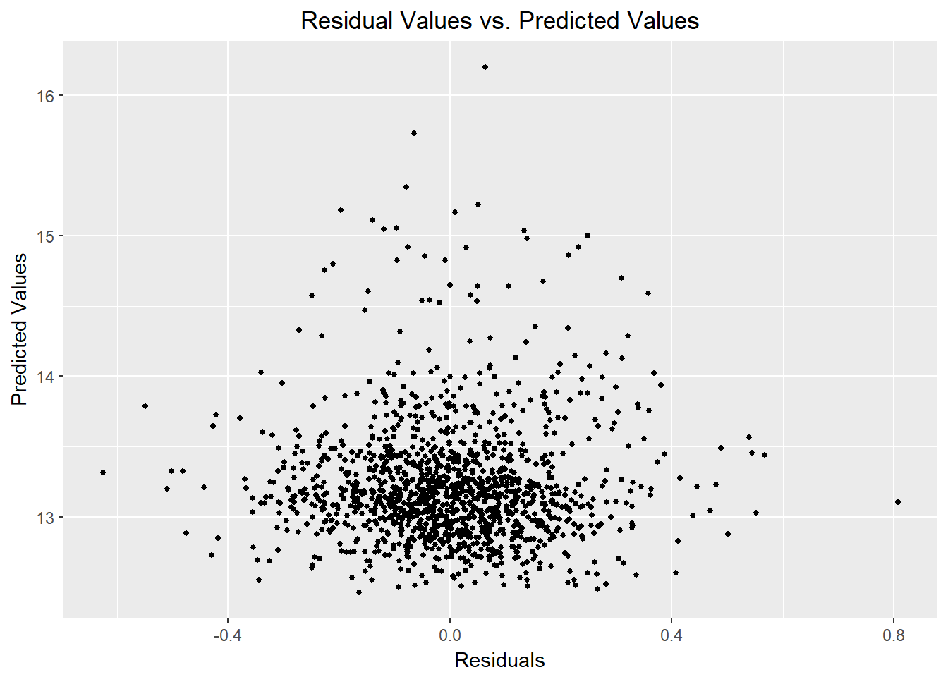
Predicted as function of observed:
regDF <- cbind(log(df_Train$SalePrice), reg3$fitted.values)
colnames(regDF) <- c("Observed", "Predicted")
regDF <- as.data.frame(regDF)
ggplot() +
  geom_point(data=regDF, aes(Observed, Predicted)) +
  stat_smooth(data=regDF, aes(Observed, Observed), method = "lm", se = FALSE, size = 1) +
  labs(title="Predicted Price as a function\nof Observed Price") +
  theme(plot.title = element_text(hjust = 0.5))
Looks sufficiently homoscedastic!
Mapping Residuals (Observation points)
reg_residuals <- data.frame(reg3$residuals)
LonLat <- data.frame(df[df$SalePrice>0,]$Longitud_1, df[df$SalePrice>0,]$Latitude_1)
residualsToMap <- cbind(LonLat, reg_residuals )
colnames(residualsToMap) <- c("longitude", "latitude", "residual")

library(ggmap)
ggmap(baseMap_invert) +
  geom_point(data = residualsToMap,
             aes(x=longitude, y=latitude, color = residual),
             size = 2) + scale_colour_gradient(low = "blue", high = "yellow") + mapTheme() +
                  labs(title="Prediction Residuals (Per Observation)")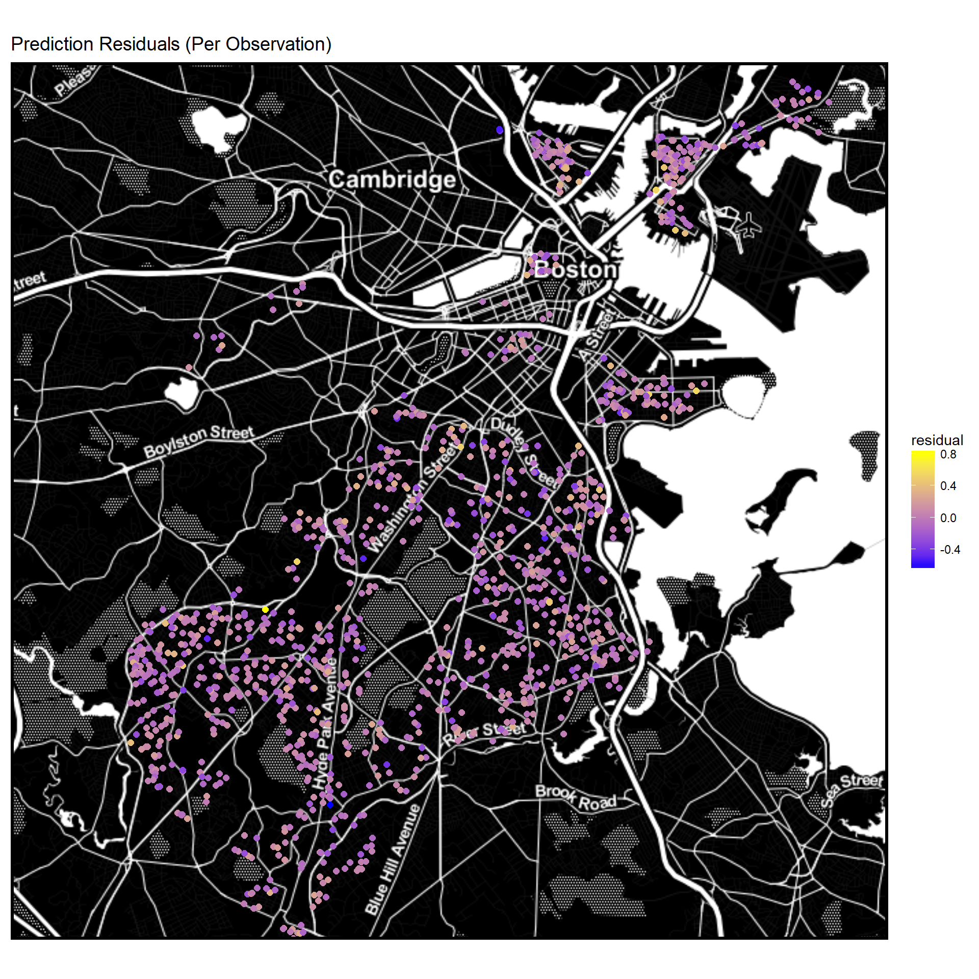
Mapping Residuals (Raster Grid Quintiles)
library(ggmap)
Raster <-
  ggmap(baseMap_invert) +
  stat_summary_2d(geom = "tile",
                  bins = 80,
                  data=residualsToMap,
                  aes(x = longitude, y = latitude, z = ntile(residual,5))) +
                  scale_fill_gradient(low = "yellow", high = "blue",
                  guide = guide_legend(title = "Residuals \n (Quintiles)")) +
                  labs(title="Prediction Residuals (Raster Grid)") + mapTheme()

Raster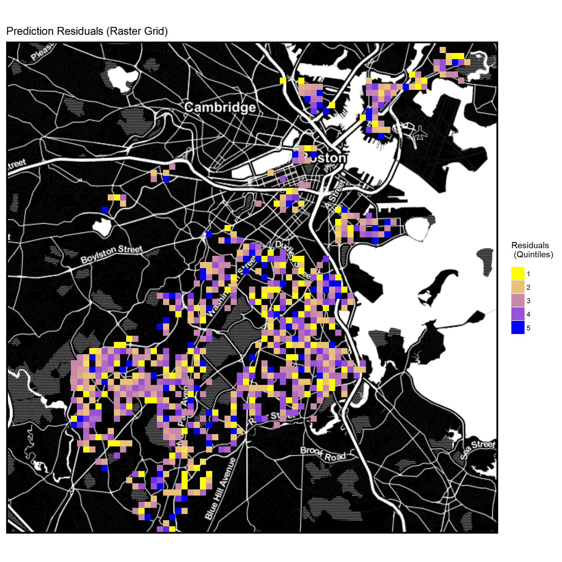
No immediately noticeable spatial pattern in residuals.
Moran’s I Analysis
library(spdep)
coords <- cbind(df[df$SalePrice>0,]$Longitud_1, df[df$SalePrice>0,]$Latitude_1)
spatialWeights <- knn2nb(knearneigh(coords, 4))
moran.test(reg1$residuals, nb2listw(spatialWeights, style="W"))
##
## Moran I test under randomisation
##
## data: reg1$residuals
## weights: nb2listw(spatialWeights, style = "W")
##
## Moran I statistic standard deviate = 0.16468, p-value = 0.4346
## alternative hypothesis: greater
## sample estimates:
## Moran I statistic Expectation Variance
## 0.0022273746 -0.0007564297 0.0003282955Test results indicate that no significant spatial autocorrelation is present in the residuals.
In-Sample Training
library(caret)
library(stargazer)
inTrain <- createDataPartition(
  y = df_Train$Neighborhood,
  p = .75, list = FALSE)

IST.training <- df_Train[ inTrain,] #the in-sample training set
IST.test <- df_Train[-inTrain,]  #the in-sample test set

reg4 <- lm(log(SalePrice) ~ ., data =  IST.training%>% #regression with in-sample training data
             as.data.frame %>% dplyr::select(-UniqueSale, -LogDist_Major_Road, -PCTOWNEROC, -DistToPoor,
                                             -DistToCBD, -SchoolGrade, -MEDHHINC, -WalkScore, -TransitSco,
                                             -BikeScore, -FeetToParks, -HEAT_SYS, -R_EXT_FIN, -R_BLDG_STY, -R_ROOF_TYP, -STRUCTURE_,
                                             -OWN_OCC, -ZIPCODE, -Style, -SaleMonth, -YR_BUILT, -R_TOTAL_RM, -NearImpBldg, -NearCommonwealth,
                                             -NearCommonwealth, -LogPCTVACANT, -LogDist_Major_Road))

#predict on in-sample test set
reg4Pred <- predict(reg4, IST.test)

reg4PredValues <-
  data.frame(observedPrice = IST.test$SalePrice,
             predictedPrice = exp(reg4Pred))

#store predictions, observed, absolute error, and percent absolute error
reg4PredValues <-
  reg4PredValues %>%
  mutate(error = predictedPrice - observedPrice) %>%
  mutate(absError = abs(predictedPrice - observedPrice)) %>%
  mutate(percentAbsError = abs(predictedPrice - observedPrice) / observedPrice)


stargazer(reg4PredValues, type = 'text')
##
## ======================================================================
## Statistic N Mean St. Dev. Min Max
## ----------------------------------------------------------------------
## observedPrice 323 619,531.800 447,474.900 245,000 3,900,000
## predictedPrice 323 608,338.200 421,368.000 260,397.700 3,890,731.000
## error 323 -11,193.530 139,614.100 -968,105.200 579,433.700
## absError 323 84,403.390 111,676.900 332.755 968,105.200
## percentAbsError 323 0.131 0.111 0.001 0.700
## ----------------------------------------------------------------------Testing Generalizability: N-Fold Cross-Validation Method
fitControl <- trainControl(method = "cv", number = 10)

set.seed(825) #set seed for random number generator

lmFit <- train(log(SalePrice) ~ ., data = df_Train,
               method = "lm",
               trControl = fitControl)

lmFit$resample
## RMSE Rsquared MAE Resample
## 1 0.1687018 0.8878129 0.1122363 Fold01
## 2 0.2279301 0.8348478 0.1483443 Fold02
## 3 0.1721422 0.8708535 0.1240672 Fold03
## 4 0.1590075 0.8361266 0.1220684 Fold04
## 5 0.1833931 0.8188797 0.1349571 Fold05
## 6 0.1714996 0.8142559 0.1328334 Fold06
## 7 0.1745891 0.8882076 0.1360352 Fold07
## 8 0.1678816 0.8672234 0.1254778 Fold08
## 9 0.1634351 0.8559889 0.1229898 Fold09
## 10 0.1546993 0.8748805 0.1234529 Fold10library(stargazer)
stargazer(lmFit$resample, type = "text")##
## =======================================
## Statistic N Mean St. Dev. Min Max
## ---------------------------------------
## RMSE 10 0.174 0.020 0.155 0.228
## Rsquared 10 0.855 0.027 0.814 0.888
## MAE 10 0.128 0.010 0.112 0.148
## ---------------------------------------The plot below shows the distibution of mean absolute error (MAE) values for the 10 folds.
#Evaluating Generalizeability: Fold MAE Frequency Plot
ggplot(as.data.frame(lmFit$resample), aes(MAE)) +
  geom_histogram(bins=5) +
  labs(x="Mean Absolute Error",
       y="Count")
No significant outliers are present
The plot below shows the per-fold R-Square statistic.
CVFolds <- cbind(lmFit$resample$Resample, lmFit$resample$Rsquared)
colnames(CVFolds) <- c("Fold", "RSquared")
CVFolds <- as.data.frame(CVFolds)
CVFolds$RSquared <- as.numeric(as.character(CVFolds$RSquared))
CVFolds$RSquared <- formatC(CVFolds$RSquared,digits=2,format="f")
CVFolds$RSquared <- as.numeric(as.character(CVFolds$RSquared))

ggplot(CVFolds, aes(x=Fold, y=RSquared)) +
  geom_bar(stat="identity", fill = "#4682b4") + scale_y_continuous(limits = c(0, 1)) + geom_text(aes(label=RSquared), vjust=-1) +
  theme(axis.text.x=element_text(angle=45, hjust=1))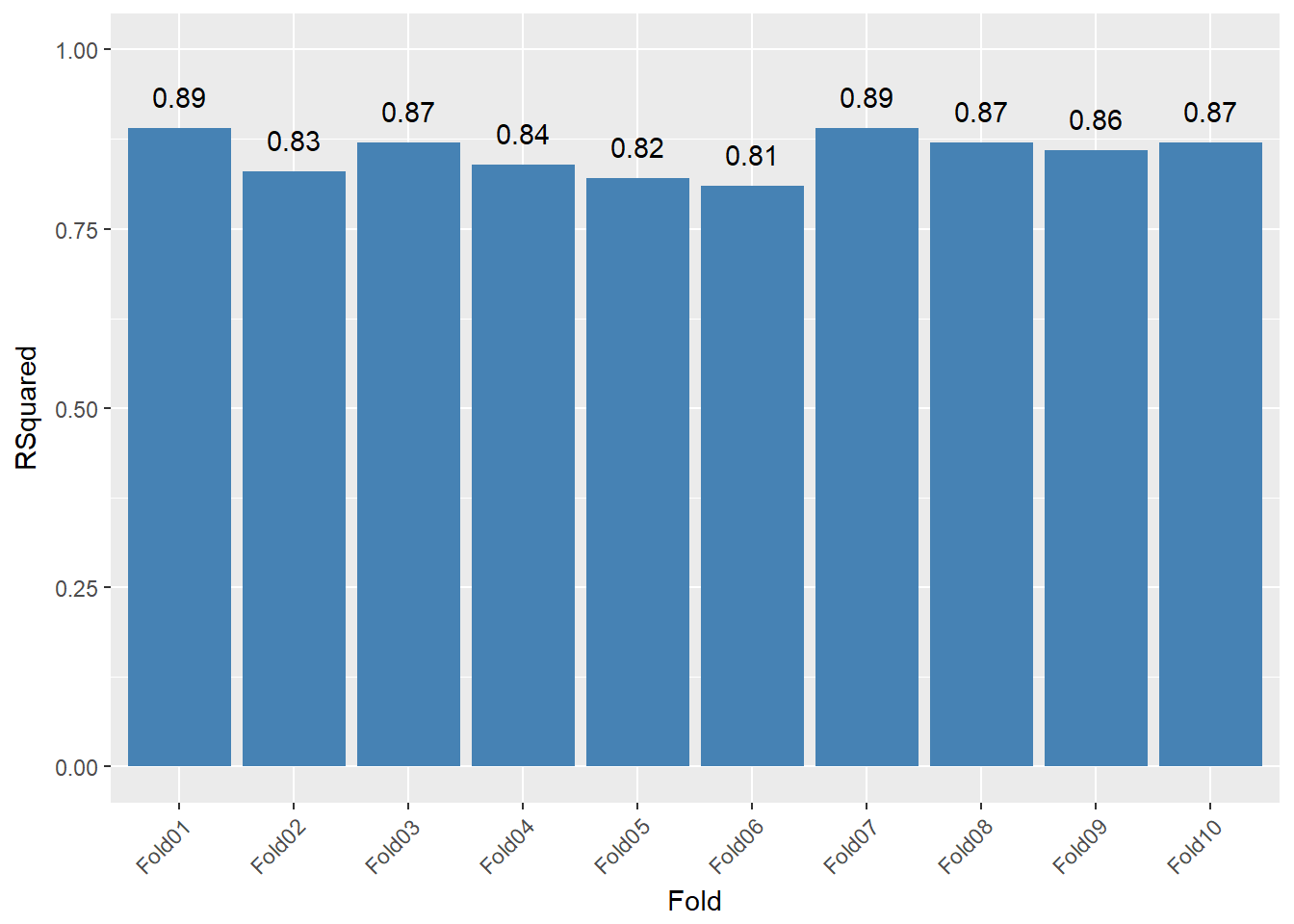
Since all folds have a similar R-Squared statistic, the model seems sufficiently generalizable.
Test-Set Predictions
The following code uses the chosen model to predict the sale prices of observations in the test set.
FinalReg <- lm(log(SalePrice) ~ ., data =  df_Train%>%
                 as.data.frame %>% dplyr::select(-UniqueSale, -LogDist_Major_Road, -PCTOWNEROC, -DistToPoor,
                                                 -DistToCBD, -SchoolGrade, -MEDHHINC, -WalkScore, -TransitSco,
                                                 -BikeScore, -FeetToParks, -HEAT_SYS, -R_EXT_FIN, -R_BLDG_STY, -R_ROOF_TYP, -STRUCTURE_,
                                                 -OWN_OCC, -ZIPCODE, -Style, -SaleMonth, -YR_BUILT, -R_TOTAL_RM, -NearImpBldg, -NearCommonwealth,
                                                 -NearCommonwealth, -LogPCTVACANT, -LogDist_Major_Road))

FinalPred <- predict(FinalReg, df_Test)

FinalPredValues <-
  data.frame(UniqueSale = df_Test$UniqueSale,
             PredictedPrice = exp(FinalPred))

head(FinalPredValues)
## UniqueSale PredictedPrice
## 3 3 625807.1
## 20 20 384205.3
## 44 44 562834.1
## 51 51 432378.7
## 76 76 471795.3
## 82 82 595516.4Mapping Predicted Values
library(ggmap)
LonLat_Test <- data.frame(df[df$SalePrice==0,]$Longitud_1, df[df$SalePrice==0,]$Latitude_1)
PredictionsToMap <- cbind(FinalPredValues, LonLat_Test)
colnames(PredictionsToMap) <- c("UniqueSale", "PredictedPrice", "longitude", "latitude")

library(mosaic)
library(RColorBrewer)
cols <- colorRampPalette(brewer.pal(5,"RdYlGn"))(5)

ggmap(baseMap_invert) +
  geom_point(data = PredictionsToMap, aes(x=longitude, y=latitude, color= ntiles(PredictedPrice, n = 5)), size = 3) +
  mapTheme() + theme(legend.position="bottom") +
  scale_color_manual(name ="Predicted Prices (Quintiles)", values = c(cols))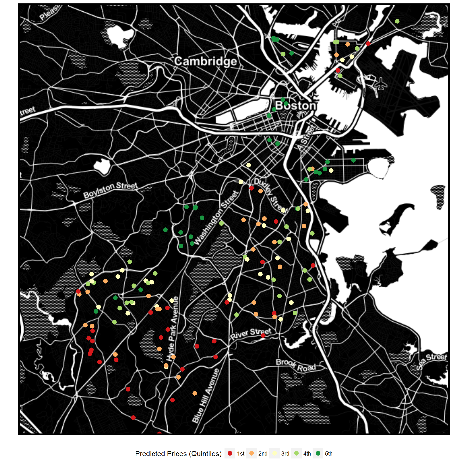
Appendix
Variable Descriptions
NewlyRemodeled - Whether the unit was remodeled since 2005 (binary variable)
GROSS_AREA - Gross floor area of the unit
NUM_FLOORS - Number of floors
R_TOTAL_RM - Total number of rooms
R_BDRMS - Number of bedrooms
R_FULL_BTH - Number of full bathrooms
R_HALF_BTH - Number of half bathrooms
R_KITCH - Number of kitchens in the structure
R_FPLACE - Number of fireplaces in the structure
SaleSeason - Season in which the sale took place. Summer= Jun-Aug, Fall = Sep-Nov, Winter = Dec-Feb, Spring= Mar-May
Style - Architectural style
LU - City’s land use designation
R_ROOF_TYP - Roof structure type: F Flat L Gambrel S Shed G Gable M Mansard H Hip O Other
R_EXT_FIN - Exterior finish type: A Asbestos K Concrete U Aluminum B Brick/Stone M Vinyl V Brick/Stone Veneer C Cement Board O Other W Wood Shake F Frame/Clapboard P Asphalt G Glass S Stucco
C_AC - Presence of central air-conditioning (binary)
FeetToParks - Distance to nearest park (feet)
FeetToMetro - Distance to nearest transit stop (feet)
MEDHHINC - Median household income of census block group
PCTBACHMOR - Percent of population in block group with bachelor’s degree or more
PCTWHITE - Percent of population in block group which identify as white
CrimeIndex - Crime ranking based on density of violent crime occurrences in 2015 (1-6)
NearUni - within one kilometer of university (binary)
SchoolGrade - ranking of nearest public school (1-9) from greatschools.com
DistToCBD - Distance to Central Business District (feet)
NearImpBldg - Whether near important landmark/building (binary)
NearCommonwealth - whether near commonwealth avenue or Boston commons (binary)
DistToPoor - Distance to neighborhoods with median household income less than 25k
NearAP - whether within 1500 feet of Logan Airport
Ave_SalePr - Average sale price of 5 nearest homes
Dist_SC - Distance to public schools (feet)
Dist_Major_Road - Distance to road with speed limit over 35 mph (feet)
LivingArea - Net living area in unit in feet (logged in model)
LAND_SF - Size of lot in feet (logged in model)